I was intrigued by the title question. So I ran a small backtest.
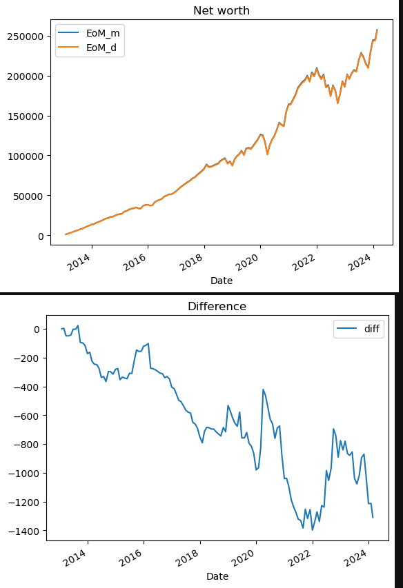
Result: no, it is not worth timing the dividends vs. naive monthly investing it by a tiny amount.
Assumptions:
- $1000 monthly budget
- only invest in VT
- time horizon: 2013+, where VT starts distributing quarterly
- $0.33 transaction fees (IB-style)
- 30% income tax applies to dividend distributions
- buy shares at End of Month. in case of the wait-for-dividends, only in case of a distribution within the month
_m is the naive monthly, _d the waiting for dividends
| A | Date | Close | feed | EoM_m | EoM_d | diff |
|---|---|---|---|---|---|---|
| 2410 | 2022-07-29 00:00:00-04:00 | 88.238220 | 1000 | 188138.655674 | 187085.197117 | -1053.458557 |
| 2433 | 2022-08-31 00:00:00-04:00 | 84.662292 | 1000 | 181514.447745 | 180547.141453 | -967.306291 |
| 2454 | 2022-09-30 00:00:00-04:00 | 76.594856 | 1000 | 165830.142229 | 165135.322705 | -694.819524 |
| 2475 | 2022-10-31 00:00:00-04:00 | 81.479149 | 1000 | 177404.305714 | 176660.973264 | -743.332450 |
| 2496 | 2022-11-30 00:00:00-05:00 | 88.227806 | 1000 | 193095.802496 | 192204.329587 | -891.472909 |
| 2517 | 2022-12-30 00:00:00-05:00 | 84.312820 | 1000 | 186506.644679 | 185729.628497 | -777.016182 |
| 2537 | 2023-01-31 00:00:00-05:00 | 90.759285 | 1000 | 201765.894238 | 200924.743411 | -841.150828 |
| 2556 | 2023-02-28 00:00:00-05:00 | 87.873535 | 1000 | 196350.542395 | 195570.322314 | -780.220081 |
| 2579 | 2023-03-31 00:00:00-04:00 | 90.378075 | 1000 | 203391.036615 | 202524.287270 | -866.749345 |
| 2598 | 2023-04-28 00:00:00-04:00 | 91.663734 | 1000 | 207283.441143 | 206404.165200 | -879.275943 |
| 2620 | 2023-05-31 00:00:00-04:00 | 90.554733 | 1000 | 205775.659521 | 204920.002602 | -855.656919 |
| 2641 | 2023-06-30 00:00:00-04:00 | 95.814117 | 1000 | 219758.410322 | 218719.893110 | -1038.517212 |
| 2661 | 2023-07-31 00:00:00-04:00 | 99.380714 | 1000 | 228936.287208 | 227858.867430 | -1077.419778 |
| 2684 | 2023-08-31 00:00:00-04:00 | 96.555099 | 1000 | 223428.566026 | 222410.814161 | -1017.751865 |
| 2704 | 2023-09-29 00:00:00-04:00 | 92.446899 | 1000 | 215579.499857 | 214684.115994 | -895.383863 |
| 2726 | 2023-10-31 00:00:00-04:00 | 89.748299 | 1000 | 210288.731464 | 209417.965008 | -870.766456 |
| 2747 | 2023-11-30 00:00:00-05:00 | 97.834183 | 1000 | 230233.627897 | 229193.387875 | -1040.240022 |
| 2767 | 2023-12-29 00:00:00-05:00 | 102.879997 | 1000 | 244425.426549 | 243211.384577 | -1214.041972 |
| 2788 | 2024-01-31 00:00:00-05:00 | 102.879997 | 1000 | 245425.096549 | 244211.384577 | -1213.711972 |
| 2804 | 2024-02-23 00:00:00-05:00 | 107.519997 | 1000 | 257491.165093 | 256180.343134 | -1310.821959 |
here the working example:
import yfinance as yf
import pandas as pd
import matplotlib.pyplot as plt
import seaborn as sns
import datetime
import numpy as np

pd.set_option('display.max_columns', None)

# Fetch historical data
vt = yf.Ticker('VT')
end_date = pd.Timestamp.now()
start_date = datetime.date(2013,1,1)
hist= vt.history(start=start_date.strftime('%Y-%m-%d'), end=end_date.strftime('%Y-%m-%d')).reset_index()
hist['yield'] = (hist["Dividends"]/hist["Open"])

# get End of Month data (will be used in purchasing & Net worth calculation)
df_EoM = hist.filter(hist['Date'].dt.to_period('M').drop_duplicates(keep='last').index, axis = 0)

# global parameters
div_tax = 0.3 # fraction of dividends you owe to the government. consider your marginal income tax rate
tansaction_fees = 0.33 # transaction fees. for IB, around 1/3rd of a $

# prepare the data. _m for the monthly staratedy, _d for waiting for dividends
df = hist.filter(hist['Date'].dt.to_period('M').drop_duplicates(keep='last').index, axis = 0)
df["cash_m"] = 0
df["distribution_m"] = 0
df["feed"] = 1000
df["shares_bought_m"]=0
df["shares_m"]=0
df["EoM_m"]=0
df["fees_m"]=0
shares_m = 0
cash_available_m = 0

df["cash_d"] = 0
df["distribution_d"] = 0
df["shares_bought_d"]=0
df["shares_d"]=0
df["EoM_d"]=0
df["fees_d"]=0
shares_d = 0
cash_available_d = 0

# let's go
for i, (idx, row) in enumerate(df.iterrows()):
    year = row.Date.year
    month = row.Date.month
    price = df_EoM[(df_EoM.Date.dt.year == year) & (df_EoM.Date.dt.month == month) ].Close.values[0] # close price at the end of the month
    div_yield = hist[(hist.Date.dt.year == year) & (hist.Date.dt.month == month) ].Dividends.sum()*(1-div_tax) # dividend yield of a month, minus tax

    # first monthly investing
    # collect cash
    distribution_m = shares_m * div_yield
    cash_available_m = cash_available_m + row.feed + distribution_m # available cash for purchase

    # buy shares
    shares_bought_m, cash_available_m  = divmod(cash_available_m,price)
    shares_m += shares_bought_m
    cash_available_m -= tansaction_fees

    # Net Worth End of Month
    EoM_m = shares_m * price + cash_available_m

    df.at[idx,"distribution_m"] = distribution_m
    df.at[idx,"shares_bought_m"] = shares_bought_m
    df.at[idx,"cash_m"] = cash_available_m
    df.at[idx,"shares_m"] = shares_m
    df.at[idx,"EoM_m"] =  EoM_m
    df.at[idx,"fees_m"] =  tansaction_fees

    # second the dividend cycle invest
    # collect cash
    distribution_d = shares_d * div_yield
    cash_available_d = cash_available_d + row.feed + distribution_d # available cash for purchase

    # buy shares
    if div_yield > 0:
        shares_bought_d, cash_available_d  = divmod(cash_available_d,price)
        shares_d += shares_bought_d
        cash_available_d -= tansaction_fees
        df.at[idx,"fees_d"] =  tansaction_fees
    else:
        shares_bought_d = 0

    # Net Worth End of Month
    EoM_d = shares_d * price + cash_available_d

    df.at[idx,"distribution_d"] = distribution_d
    df.at[idx,"shares_bought_d"] = shares_bought_d
    df.at[idx,"cash_d"] = cash_available_d
    df.at[idx,"shares_d"] = shares_d
    df.at[idx,"EoM_d"] =  EoM_d
df["diff"] = (df.EoM_d-df.EoM_m)

df.plot(x="Date",y=["EoM_m","EoM_d"],title="Net worth")
df.plot(x="Date",y=["diff"],title='Difference')
keepcols = ['Date', 'Close',
      'cash_m', 'distribution_m',
       'feed', 'shares_bought_m', "fees_m", 'shares_m', 'EoM_m', 'cash_d',
       'distribution_d', 'shares_bought_d', "fees_d", 'shares_d', 'EoM_d', 'diff']
df[keepcols].tail(20)
follow-up question:
- 2013-2024 is one of the strongest bull markets in history. would we have the same results in a sidways-or bear market?