Statistics, black magic and financial mathematics

Yeah, this is “continuous” in this context.

No, this statement indicates that you are always “playing with the whole bankroll”. Has nothing to do with the length of the time step.

The modern portfolio theory assumes log-normal distribution of returns. This is what I was trying to acquire.

Let’s have a bit more fun!

To classify the state of the stock market, as quantified by a specific index, I am going to consider these five regimes:

  • Normal State: the market index is less than 5% below its all-time high (ATH).
  • Mild Correction: the market index is between 5% and 10% below the ATH.
  • Correction: the market index is between 10% and 15% below the ATH.
  • Deep Correction: the market index is between 15% and 20% below the ATH.
  • Bear Market: The market is in a ‘Bear Market’ regime when the index drops more than 20% from the ATH.

These regimes can be utilized, for example, to define different portfolio consumption rates, adapting them to the current market conditions.

And I hope I won’t need to define a ‘Deep Bear Market’ any time soon.

From here:

I’d love a discussion between him and RR folks on this topic. :smiley:

You mean him and Ben? :wink:

Yeah, with Benoit, but also with some of their guests vouching for SCV.

There are some podcasts linked in the original post, so maybe it has happened already.

For all calculation freaks: here you can download LIK/Swiss CPI index values with an insane precision of up to 7 numbers! All bases and 12 month changes in the same file.

P.S. Updated to 03.12.2025 version. The link for the newest version of the file is changing every month, but you can always browse to the page with it.

What values to use to analyze long-term return of equities? My answer.

Source: Elroy Dimson, Paul Marsh, Mike Staunton. Credit Suisse Global Investment Returns Yearbook 2023, Chapter 2, Table 1, page 16 in Summary Edition.

Annualized real equity returns over the last 123 years for the “World index”:
Arithmetic mean: 6.5%
Standard deviation (volatility): 17.4%

These values translate nicely to
Geometric mean (CAGR): 5.0%

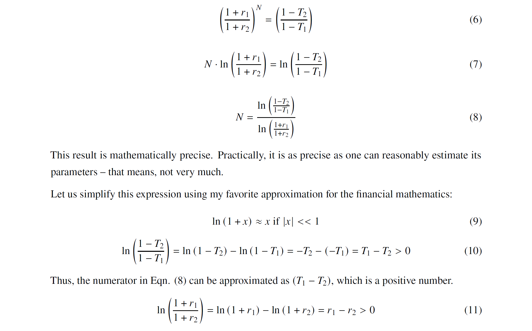
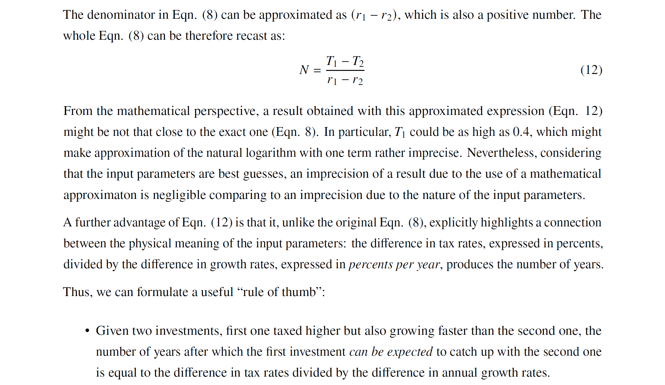
I have seen 5% often used as an estimate of a long-term real return of equities, but without much justification. I guess most used this number for convenience and simplicity, but it also appears to be a good choice.

You can plug these values into a Monte Carlo simulation tool:

https://www.portfoliovisualizer.com/monte-carlo-simulation

Parameter Value
Portfolio Type: Asset Classes
Inflation Adjusted: No
Tax Treatment: Pre-Tax
Simulation Model: Parameterized Returns
Distribution: Normal Distribution
Expected Return: 6.5
Volatility: 17.4
Sequence of Returns Risk No Adjustment
Inflation Model Parameterized
Inflation Mean 0
Inflation Volatility 0
2 Likes

I stopped reading here.
But thanks.

Edit: Well actually it’s interesting and simple to understand even for me.
Thanks again.

Credit Suisse was and UBS is just a sponsor of a yearly publication by Elroy Dimson, Paul Marsh, Mike Staunton. It is really worth reading, and somehow especially 2023 edition was “back to basics”.

Maybe it is just my impression because it was the first such Yearbook that I read, but I couldn’t find a reproduction/update of that Table 1 that I refer in 2024 and 2025 editions.

2 Likes


3 Likes