Also the +/-34% rule is only applicable to normal distributions, the cumulative distribution function of a lognormal will be very different and certainly not symmetric.
Sure. + and - sigma intervals become * and / by factor 10^sigma. So it would be more correct to say that with a 68% probability the annual “relative” return is between 1.0905/1.184 = 0.921 ( -7.8% ) and 1.0905*1.184 = 1.291 (29.1 %). But I don’t see here any percentual value that I could call “annual volatility”.
Is it (29.1%+7.8%)/2 = 18.45 %? As expected, it is basically the same as I calculated above.
Yes but it is not relevant here.
I am talking about ±sigma levels of normal distribution of logarithm of the return. If we recalculate X-scale, 68% of possible outcomes is still located between these two levels recalculated to a new X-scale.
My question remains: what is volatility? Or better: how financial folk calculates volatility and since we are at that, how do they calculate annualized return/CAGR/whatever?
What do you guys mean?
Isn’t volatility ~ variability (over time) ~ literally variance or stddev (sqrt of it)?
I am no statistician, I was just assuming this all my “financially aware” life.
No statistician either, but I think the question is legitimate, you cannot simply calculate the standard deviation of the variable over time if it’s following an underlying non linear growing curve like we expect for the stock markets.
I’ve always assumed you could use the standard deviation of the returns themselves. However if the returns are lognormally distributed as @Dr.PI suggested it’s possible that the definition might not be as straightforward as I thought.
Ok, after a quick search it seems that at least W. Sharpe (the one of the Sharpe ratio) was indeed using the simple standard deviation of returns (actually of differential returns compared to a benchmark, but the idea is the same) as a measure of risk. So nothing too hard and his definition is very clear.
I’m sure there’re more refined models out there that estimate volatility while accounting for different distributions but I guess in first approximation this should be good enough.
Looks like the most common way to calculate volatility is to calculate standard deviation of daily (percentual) price/value changes and then scale it up to 1 year, i.e. annualize.
Help me figure out the Target Volatility formula - Bogleheads.org
The Portfolio Visualizer FAQ says:
The target volatility model uses dynamic asset allocation to achieve a stable level of volatility. … The model calculates the realized portfolio volatility (annualized daily volatility) based on daily total returns.
And this guy says that it is enough to look at the last 20 days to calculate (current) volatility, which is an annualized standard deviation of daily percentual returns:
A measure of the volatility of a fund — based on the fund’s last three years of monthly returns — used to indicate the dispersion of past returns.
So, they calculate a standard deviation of monthly percentual returns and scale it to a one year period. They do it to be able to compare with the volatility of the benchmark index, which is calculated once per month (or at least monthly values are more reliable, I guess).
In their index factsheets MSCI also quotes “ANNUALIZED STD DEV” with a note “Based on monthly price returns data”.
So, it looks like the volatility is a robust parameter and you don’t need much to calculate it.
I started from an assumption that the expected “relative” return on an investment over some time frame N, X = P(t)/P(t-N), follows a log-normal distribution, and now I am talking about the standard deviation of “percentual” returns. But there is no contradiction.
If we now take a natural logarithm of the “relative” return X, ln(X), we expect it to be normally distributed. If we now transform it:
X = P(t)/P(t-N) = [P(t) - P(t-N) + P(t-N)] / P(t-N) = 1 + [P(t) - P(t-N)] / P(t-N) = 1 + x
where x = [P(t) - P(t-N)] / P(t-N) is precisely a relative change of the value, i.e. a “percentual” return.
Now we know from the math that ln(1+x) ≈ x if |x| << 1.
So, if ln(X)) = ln(1+x) is normally distributed, than x follows exactly the same distribution if x is small. Daily and even monthly variations are typically within 10-20%, so we are fine here.
But if we are talking about a long time frame (or, as a side note, about an extremely volatile price), we should not forget that relative returns are log-normally distributed.
(to be continued)
So let us define a “return ratio” as a change of price/value of an investment P(t) after a certain time period:
X = P(now)/P(past)
As was already said before, due to the continuous compounding, the expected return ratio on an investment follows a log-normal distribution. According to a definition, variable X follows a log-normal distribution if ln(X) follows a normal distribution. A normal distribution is given by:
Here μ is the mode, median and mean of the distribution and the expected value of the variable x;
σ is the standard deviation;
σ^2 is the variance of the distribution.
Let’s say that a return ratio X over one period follows the log-normal distribution with parameters μ1, σ1 and variance Var1=σ1^2. Let’s further consider a single asset with a constant return rate and volatility, which means mathematically that μ and σ of the log-normal distribution remains constant from one period to another. Due to the compounding, return ratios over multiple periods are multiplied, which also means that ln(X) is adding up. If for each period the distribution of the probability remains the same, then after N periods we obtain:
The parameters of the distribution μ and σ are usually not calculated from a 1 year return ratios/changes. Instead, they are annualized: scaled by a number of periods that correspond to one year. If parameters are calculated from 1 day change, then one takes N equal to a number of trading days in a year (e.g. 252); if they are from 1 month changes, one takes N = number of months in a year, etc. Now we obtain a (log)normal distribution with annualized parameters, which describe distribution of return ratio after 1 year.
σ_ann is an annualized volatility, and this is what is quoted in a description of an asset. But there is no annualized mean return. Instead, a “compound annual growth rate” (CAGR) is given. They are related as following:
Now let’s say that an initial investment with constant annualized volatility and CAGR is left to compound returns for Y years. What is the statistic of the return ratios?
X = P(t)/P(t - Y years)
A probability density function of the log-normal distribution of return ratio after Y years is
Cumulative distribution function is, unsurprisingly
And now some interesting levels:
You have a 50% probability to obtain the median return ratio:
Your most probable (highest probability) result is the mode return ratio, which is less than the median:
Your mean (expected) return ratio is:
The relation between the median and the mean return ratio is
You would have gotten the mean value of the return ratio if you returns would add up instead of compounding. In this case you would get another, “arithmetic” annual growth rate.
The difference between “arithmetic” and “compounded” growth rate seems to be the famous volatility drag. See for example
You have 99% probability to get a return ratio of at least
90% probability to get at least
67% probability to get at least
33% probability to get at least
10% probability to get at least
1% probability to get at least
And that was a story of a single asset with constant return rate and volatility. It is relatively simple, but already gives an idea how return rate and especially volatility affect the return on the investment.
I think I learned a lot from https://breakingthemarket.com/ blog, which explains investment-related mathematics in a way accessible to me.
Well, when I read it deeper I realized that even a story of one asset is not so simple. First, we should distinguish between “arithmetic” and “geometric” rates of return. Both are “real” enough to (earn/lose extra) profit from. The relation between them is
So the geometric return rate is less by the “volatility drag”.
I went back to SPI data and look at the rate of returns over even longer periods. Graphically, the histograms of ln(return ratio) look very good for 1, 5, 10, 21, 42 days; for 63 and 126 days it starts to look not like a Gaussian; for 252 and more days it has many subpeaks. Nevertheless I calculated annualized return rate and standard deviation for all distributions and this is what I obtained:
My interpretation is following: for time intervals up to 21 days we are still in the “arithmetic” range of return rates. This time is not long enough for interest to start compounding, our investment have no “memory” yet. Starting from few months, the rate of return decreases. Arithmetic return rate of 9.18% and annualized stddev 16.6% (calculated as an average for 1-21 days results) transforms to 7.8% geometric return rate. The actually calculated return rate is not decreasing that much, but it is still half-way there.
I might take a look at the other data, but I don’t expect significant qualitative changes.
So, (arithmetic) return rate and volatility are two characteristics of an asset, which are of importance for us. Ideally one would like to invest in an asset with high return rate and low volatility. But there are no free lunches: assets with higher returns have higher volatility. Fast forward: the most important message I took out of the blog is following:
A rational investor should at every moment of time maximize expected geometric return!
Here r_arithm is now the expected arithmetic return rate of the whole portfolio, σ^2 is the variance of the whole portfolio.
This might be a highly abstract theoretical concept, but if you dig deeper into it, you have everything that is being said about investing:
Asset allocation
Weakly-correlated assets
Rebalancing
Leveraging
I will continue with some applications of this formula, and for now would love to have a feedback.
You’re unlikely to get very far with your ‘annualized’ volatility assumption, be it based on some historical rolling average or not.
In reality ‘market’ or ‘portfolio’ volatility (however that my be defined) bounces up and down continuously. The literature is full with difficult mathematical models trying to model that (and fail).
Therefore I gave up trying to understand these models long ago and use them to my advantage. Instead I pick an average tracker
Although the guy behind breakingthemarket.com seems to have build an outperforming investment strategy, this is not my goal. My goal now is to better understand a theory of investment.
In general I don’t like just to be told what is the right way, but prefer to understand and figure out myself why it is the right way. On the other hand I also don’t want ignore existing knowledge and do lots of trials and errors with my actual investments; to perform “real-time” simulated trading I want even less. So I decided to go with a simple and well-established “total stock market” investment strategy while learning the theoretical framework.
“Maximizing geometric return” looks like a simple theoretical framework with extensive conclusions. It should help to understand why one should do certain things and why certain things should be avoided.
So, now let’s say we have a portfolio containing certain assets 1,2,…,n and we try to maximize our future profit by maximizing expected geometric return via a proper allocation of these assets with weights w1, w2, … wn (sum is 1). Weights can be also negative, meaning we are short-selling an asset or borrow cash.
How can we do this?
We can find a theoretical answer with a help of so called “Modern portfolio theory”. General Wikipedia have a very comprehensive description
We have to calculate two things: an expected (arithmetic) return rate r1, r2, … rn and a covariance matrix Σ. Covariance of two distributions in statistics is the expected value (mean) of the product of their deviations from their individual expected values.
Let’s say we have historical data for two assets P1(t) and P2(t). Here is a small example how we would calculate (historical) return rates and covariance between these two assets:
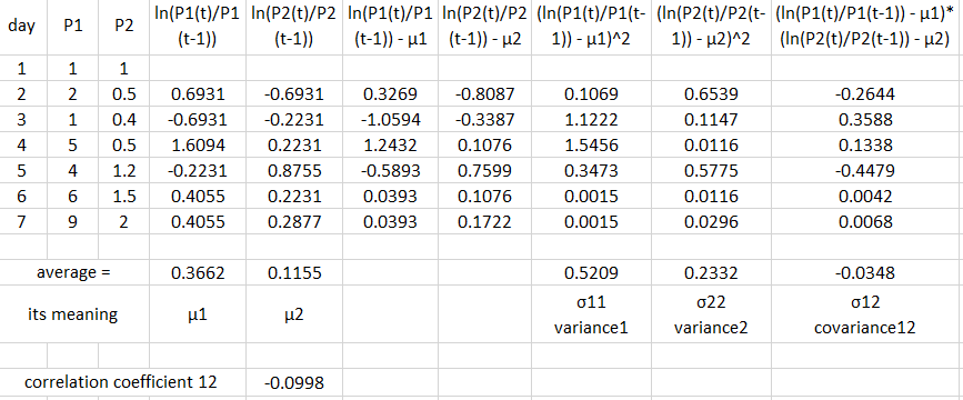
First we need price data for 2 assets (P1 and P2). Each row corresponds to values of P1 and P2 at the same moment, e.g. closing prices/NAV in the same day. Then we calculate ln(return ratio), here after one day, for both prices. The average of values in individual rows is the mean of lognormal distribution of return ratios μ1,2. As a next step, we need to calculate a deviation of individual ln(return ratio) from its mean value, (ln(return ratio)-μ). If we now square these deviations and calculate average value of the results, we obtain the variance of returns for respective assets. But if we multiply deviations for different assets and calculate average of the results, we obtain a covariance of returns for assets 1 and 2. In this case it is negative, meaning that on average prices of 1 and 2 go into opposite directions.
Note that one should probably annualize mean return and mean co/variances by multiplying obtained values by a number of periods corresponding to a full year, and calculate an arithmetic annual return rate r = exp(μ)-1.
While co/variances is all we actually need, it is interesting to look at a correlation coefficient for two assets. It is given by
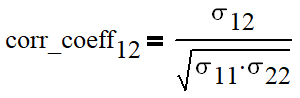
The value of the correlation coefficient is limited and lies between -1 and 1. It is 1 if asset changes are always go in one direction, 0 if changes are completely independent and -1 if they always go in opposite directions. In this case the value of the correlation coefficient between 1 and 2 is slightly negative, meaning that in average the prices of two assets change rather in opposite than in the same direction.
Back to the covariance matrix Σ: for assets 1,2,…n, the element of the covariance matrix Σ(i,j), 1 ≤ i,j ≤ n, is equal to the covariance of assets i and j. Every diagonal element (i=j) is a covariance of the asset i with itself, that means, variance.
The expected (arithmetic) return of the portfolio and its variance is best calculated using vectors and matrices. Let R and W be vectors containing annualized expected returns and weights of respective assets in the portfolio:
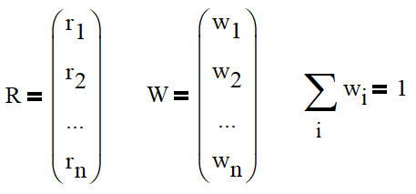
The covariance matrix contains annualized co/variances calculated as outlined above.
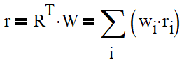
The expected (arithmetic) return of the whole portfolio is then simply a weighted average return of all assets:
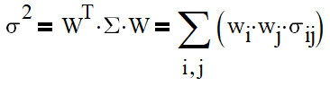
The variance of the whole portfolio is given by the following formula:
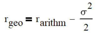
Finally, our tasks consists of finding weights of assets that maximize the geometric return of the whole portfolio:
And that was a general theoretical description of a multi-asset portfolio.
Now let us consider a special case of a multi-asset portfolio: one asset with varying returns and cash.
The asset is characterized by an annualized arithmetic return rate r1 and variance of returns σ1^2. Note that it does not have to be a really single asset, it can be also a (sub)portfolio with given parameters. The weight of this asset/subportfolio in our portfolio is w1.
Cash is characterized by a constant annualized return rate r2 (risk-free rate). As it is constant, cash has variance of 0, covariance with any other asset is also 0. That’s why an addition of cash does not bring any “cross-talks” into our risky subportfolio, which can be considered as a single asset. The weight of cash is w2=(1-w1).
Using formulas for return and variance of multi-asset portfolio, we obtain
And the geometric return is:
The latter as a function of w1 gives us a nice parabola with a maximum located at
which gives an optimal allocation of the risky asset in the portfolio.
Well, the theory was fun. Now back to tough reality.
I have been taking rather bad parameters for stock market returns (annualized volatility 20%, expected annual return 6%) and calculating an optimal asset allocation for a given interest rate on CHF cash deposits. With an interest rate of 2% on cash, the optimal allocation is 100% stocks. With the same bad returns on stocks and a cash interest rate of 3%, one obtains 75% stocks as an optimal allocation.
Nowadays, it is tricky to get more than 0.3% on CHF deposits. 1% would be a guaranteed minimum interest of the second pillar, 3% is a very good long-term return of the second pillar. Unfortunately the return of the second pillar is not really constant, and it is not necessarily (anti|un|)correlated with the stock market returns. Also reductions of taxes should increase the “interest rate” of the second pillar, but here it is not accounted for.
So, the conclusion about the cash-stocks allocation under current conditions is unfortunately following: 100% stocks, but putting some cash into second pillar (if you have a good one) in years of strongly rising stock markets won’t hurt.
If the interest rate on cash is less than 2%, the formula for an optimal asset allocation gives stocks weighting of over 100%. It means that the theoretical framework suggests us to borrow cash at a rate r1 and buy stocks with the borrowed cash. In this case, one should replace “deposit” interest rates with “borrowing” interest rates. But still, if one borrows CHF at a rate below 2% (e.g. via mortgage), it is very attractive to somewhat leverage the portfolio.
Understanding volatility of portfolio composed of few assets is not so straightforward, but we can illustrate it quite easily, at least for 2 assets.
So, we have a portfolio containing 2 assets with weights w1 and w2 = (1 - w1), which are characterized by annualized volatilities σ1, σ2 and respective variances of returns σ1^2 and σ2^2. The correlation coefficient between assets 1 and 2 is ρ12. The variance of the portfolio is given by
Namely, if (in 2D) we have two vectors with lengths L1 and L2 with the angle α between them, the length of the sum vector L is given by
Now we can make an analogy. If the volatility of an asset σ1, σ2 is the length of a vector V1, V2 and the angle between the directions of two vectors is given by α = arccos(ρ12), then the volatility of portfolio σ_tot is just the length of the weighted sum vector:
As we change the portfolio composition, the end of the sum vector representing σ_tot is moving along the straight line connecting ends of two vectors representing σ1,2 (blue line).
Geometry tells us that the lowest length of the sum vector (red) corresponds to the portfolio composition that produces the sum vector perpendicular to the blue line.
So, if the volatility of two assets is exactly the same (σ1 = σ2), the 1:1 portfolio will have the lowest σ_tot no matter correlation coefficient/angle between the vectors, which is equal to
If the angle is small/correlation coefficient is high, this lowest σ_tot is very close to σ1,2; if the correlation coefficient is low, σ_tot could be significantly lower.
Now, if σ1 and σ2 differ, geometry tells us that the lowest σ_tot corresponds to an intermediate asset allocation only if the ratio between the smaller and the larger volatility is less than cos(α) = ρ12; otherwise it corresponds to 100% of the asset with the lowest volatility. If the correlation coefficient is high/the angle between two vectors is small, there is hardly any chance to significantly reduce total volatility by changing weights of the assets.
Here is an example for α = 45°, an angle that almost exactly corresponds to ρ12 = 0.7. Around this value of the correlation coefficient one can expect a reasonable reduction of σ_tot in comparison to σ1,2, but only if the ratio between the smaller and larger volatility is less than 0.7.
One can easily see that with ρ12 > 0, α < 90° the lowest possible σ_tot is in general rather close to min(σ1,σ2). Things are getting really interesting if ρ12 < 0, α > 90°. In this case, it is possible to obtain low σ_tot even if both σ1,2 are high. Taking ρ12 = -0.5, α = 120° as an example:
Nice idea, because nominal stock returns can be misleading, especially in your decumulation/retirement phase. Stock market gaining 2% doesn’t mean you got 2% more spending power if inflation’s risen by 2%.
Someone should inform cash/bond investors too who get excited about their nominal interest rates
By reading and partipating to this forum, you confirm you have read and agree with the disclaimer presented on http://www.mustachianpost.com/
En lisant et participant à ce forum, tu confirmes avoir lu et être d'accord avec l'avis de dégagement de responsabilité présenté sur http://www.mustachianpost.com/fr/
Durch das Lesen und die Teilnahme an diesem Forum bestätigst du, dass du den auf http://www.mustachianpost.com/de/ dargestellten Haftungsausschluss gelesen hast und damit einverstanden bist.