I heard this quote one too many times and it made me want to check (and it’s your fault, @Compounding ![]() ). Could the equity premium really be so undefined that statistics only tell you it is between 10% or 1.5% (with 95% confidence)?
). Could the equity premium really be so undefined that statistics only tell you it is between 10% or 1.5% (with 95% confidence)?
When I talk to investment advisors, I love to ask them, “What is the equity premium?” I get a range of answers, but almost everyone thinks it’s somewhere between 4 and 7% and 6% is what I hear most. Then when you ask people where they come to that number, they say, “Well, you look at the last 100 years and it’s been 6%.”
That’s true. If you look at 100 years of data, you see a 6% equity premia, but if you get that mean equity premia by running the regression, it also gives you a confidence bound on your estimate. It turns out that the estimated equity premium that you get by looking at the past data is 6% plus or minus the standard deviation of like two and a quarter percent.
So, if you just are a frequentist probablist, you do the frequentist statistics, you’re basically saying you’re 95% sure that the true equity premium is between one and a half percent and 10 and a half percent. You just have no idea. With 100 years of data, we can’t come close to agreeing on what the equity premium is.
on Rational Reminder Podcast
Now, I don’t claim I’m cooler than a bona fide professor, but with a century of nearly daily closing data, this got to be more precise.
So, I ran my own regression in Libreoffice Calc (opensource Excel). I set it up according to this tutorial. I only changed the calculation of t, so it would actually take df instead of a hardcoded 13. I verified that I got the same numbers as on the tutorial screenshot. The tutorial also uses 95% confidence, so that should be appropriate.
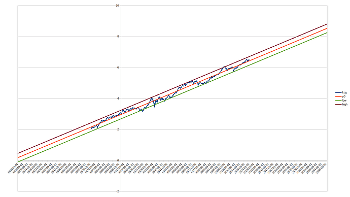
Then I took the monthly real total return of the US stock market from https://shillerdata.com/. The dataset spans from 1871-01 to 2024-03. That contained 1839 months. Assuming exponential growth, I applied the log-function to all prices. With this I can then run the simple linear regression from the tutorial.
I undid the logarithm by exponentiating again on the mean, high and low predictions. Then I just calculated:
- mean=last\_mean/first\_mean
- max=last\_high/first\_low
- min=last\_low/first\_high
As a last step I annualized them:
- f(r)=r^{\frac{365}{55942}}
I get:
- mean=6.62\%
- max=7.51\%
- min=5.74\%
And those are even slightly too far apart, since tangents should have been used.
Here a log plot. The predictions outside the data interval don’t even visibly diverge anymore because there are so many datapoints.
I also tried with just yearly data, but the picture doesn’t change much.
I can’t find the 2.25% standard deviation. So, what did he mean here?
