Need to sell 25% of my portfolio

I need to sell 25% of my stock market portfolio over the next 2 years to fund my pension and pay for renovations. So far, I’ve been selling in the last quarter to fund pension, so if I stick to what I’ve been doing, I would sell 13% in Q4 2025 and then 12% in Q3 2026 (when the renovations will be done).

But I wonder whether it is more prudent to sell now as it is a short-term need and so the stock market is probably not an appropriate place to park the funds.

What would you do?

I think if I were you, I would calculate how much money I need to take out from stocks over next 5 years and ensure that much money is not in stocks already. It should be in cash, duration matched bonds, etc.

Given the high volatility of equities, typical hold period is 7-10 years. So this should be valid at any point of time irrespective of how long the money is already in stocks. Time always starts to count “now”.

If you think about it , if someone would come to forum and say , I have 200K in cash but I need it in 2 years, where should I invest it to maximise returns?

The answer on forum will be -: fixed income :slight_smile:

6 Likes

I would sell now the amount and buy an ETF like BSV until I actually need the money.

Would you be comfortable to sell 33-50% of your „current“ portfolio? If not, I would hold the required amount in cash. I know the opportunity costs might be huge, but so are the risks.

1 Like

Definitely bonds.

I’d personally buy two tranches of US treasures maturing around the time you need the money and accept the currency risk.

If you don’t want to accept the currency risk, hedge, or accept lower yielding CHF government bonds or so.

1 Like

I forgot to mention, the portfolio yield is a bit above 4%, so I guess, I’d take the income and then only have to sell around 9% and 8%.

Portfolio is in USD and expenditure will be in CHF, so there’s also currency risk. Though I’m OK with that.

1 Like

US treasuries still yield around 4% for your planned time periods and are as risk free as it gets. If the US won’t pay you back, the world has different problems that probably make your planned investments moot …

If you need the money in CHF in the shorter term, parking it in an USD money market fund is a really bad idea.

Risk free only as an US investor, having expenses in USD.

Just look at CHF/USD volatility over the last years.

We went from 1:1 to 1:1.20 back and forth.

That‘s massive.

4 Likes

I get that there’s currency risk, but I believe @PhilMongoose just mentioned he’s ok with that.

Hmm. Apparently Past_Phil had his shit together and actually did buy a bond to cover his 2026 expenses. So that just leaves the 2025 payment that needs funding.

EDIT: Apparently, he also bought a bond for 2025 too, but Current_Phil (aka Chump_Phil) forgot what it was for and sold it and bought Gold with the proceeds.

12 Likes

Change the topic title to: “Here is one weird trick to un/re-cover the unknown or forgotten 20% of your portfolio that you didn’t know about …”

:wink:

BTW, the thread participants here demand and deserve a 10% finder’s fee.
Send it to my beetcoin address and I’ll make sure it gets evenly justly distributed among the participants here.

1 Like

An option could be to place trailing stop-limit orders on what you intend to sell; that gives downside protection, but participation to upside if any.

It doesn’t provide any protection in case of gap down scenarios.

1 Like

Something like IVVB (protection for 15% downside per quarter, but max 5% upside) or IVVM (5% downside, 5% upside cap)?

1 Like

Suddenly appearing short-term obligations on long-term portfolios are very suboptimal. It’s 25%, but if the market crashed earlier, it could have been 50%. And it still can be.

If you can not delay this in case the market turns sour, you might take a long-term hit. The underlying reason is that we are affected by geometric instead of arithmetic returns. Let me explain:

Model and Example

Let’s assume our portfolio can increase by 2x or shrink by its inverse (0.5x) with a 50-50 chance (we call this a) It could be other numbers, but the point is that this portfolio has an expected return of 1 (geometric return, instead of 1.25 like arithmetic returns would suggest), because we are forced to run those coin flips in series, all-in.

A long-term portfolio should also have return (maybe 1.05, and we call it c) above the risk free rate (which we will assume to be 0% and matching inflation for simplicity’s sake).

Now, we know we will have a fixed expense at a point in the future. It is some percentage (25%) of our portfolio at present (called b). We can choose to convert to the risk free asset now or later.

General formulas:

now later
up
(1-b)*a*c a*c-b
down
(1-b)*\frac{1}{a}*c \frac{1}{a}*c-b
Geometric
Expectation
(1-b)*c ((a*c-b)*(\frac{1}{a}*c-b))^{0.5}

Numbers

now later
up
1.575 1.850
down
0.394 0.275
Geometric
Expectation
0.788 0.713

We see that the return of converting later is much reduced. The additional return from our portfolio couldn’t overcome this.

All coin flips

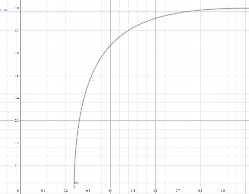
But maybe an a of 2x/0.5x movement is a bit extreme. Lets draw a curve over all a:

The advantage at low volatilities is small, and reaches 0.788 vs. 0.800 in favor of “later” at no volatility (= 1). And of course, at 4x/0.25x the 4x means nothing, because you risk getting wiped out.

Analytical solution

I tried to calculate this with a over a log-normal probability distribution. But since that includes the chance of falling to 0.25 and below the geometric expectation is 0. This is where this model reaches its explanatory limits.

But this does mean that for example using leverage without protections will at some point bankrupt you. Though, depending on the likeliness, that could take much longer than you have time to live (or the whole of humanity for that matter). If your capital has more than one heir, the new capitals will be insulated from each other. At that point this turns into arithmetic returns, where some total failures can still have a positive expected return over all portfolios.

Monte Carlo

So, I ran a Monte Carlo simulation (n=100’000) over 4 quarters with log-normal distributions with μ=0, σ=0.096 (quarterly standard deviation of S&P 500 Price since around 1928), and applying the functions from before,

now(x_1,x_2,x_3,x_4)=(1-b)*x_1*x_2*x_3*x_4*c
later(x_1,x_2,x_3,x_4)=x_1*x_2*x_3*x_4*c-b

and also their combinations, e.g.:

semi(x_1,x_2,x_3,x_4)=(x_1*x_2*c^{2/4}-b)*x_3*x_4*c^{2/4}

Additionally there is a roll strategy, which makes five equal sized buckets and allocates them to one strategy each, over the same 4 quarters.

This gave me the following metrics:

now​ quarter semi 3-quarter year roll
MIN 0.375 0.330 0.294 0.281 0.251 0.309
MAX 1.701 1.822 1.903 1.947 2.017 1.872
AVERAGE 0.802 0.807 0.811 0.815 0.819 0.811
GEOMEAN 0.789 0.790 0.792 0.794 0.796 0.793
STDEV 0.149 0.163 0.176 0.188 0.198 0.174

Discussion

Based on these numbers, the additional return of could rationally be worth the additional volatility. This seems to be in line with normal leverage (with which it has much in common). We also see that “roll” slightly improves over “semi” in both GEOMEAN and STDEV.

The most extreme yearly drawdown I found in the SPYTR data of testol.io was -68.50% on 1932-06-28. Subtracting an additional 25%, would have left the portfolio at 6.5%. The stock market isn’t a log-normal Monte Carlo simulation. But you aren’t a robot either, and wouldn’t liquidate for renovations on that day.

To be honest, I didn’t expect that liquidating later would have the better expected geometric return. And for portfolios of higher volatility, or with less return, or if the expense is bigger, it doesn’t. But for those reasonably chosen values it works.

tl;dr: Selling later or rolling seem to be superior in return to selling now. This was calculated on a model with assumptions and not historical data.
13 Likes

This is quite some work. Awesome.
I tried to grasp this completely but still have questions to understand the numbers

These expectation numbers are probabilities of having higher return or they are the actual returns?

For example in Monte Carlo simulations

Average is 0.802 for now and 0.815 for later, what does this actually mean?

80% chance to have a better return or 0,8% is the access return?

I don’t think this is correct. I think the expected return is 1.25. If you think otherwise, I’m happy to play a repeated coin flipping game with you where I give you 50 on heads and you give me 100 on tails until one of us is convinced :wink:

-50% and +100% of everything each participant has, repeatedly. After some time we stop and invest in a constant low rate investment. The average time to reach an arbitrary net worth has stayed the same (or even increased since some series are needlessly above the goal).

Where your whole portfolio is concerned, calculating arithmetic returns paints a misleading picture.

1 Like

Those are the actual final value of a portfolio. The portfolio starts with 1.000.

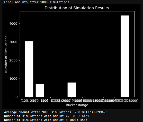
I ran a simulation (see below). As expected, about half fall below the starting amount and half fall above.

You are right that looking at average time to hit a target will be the same since chance of double/half was equal.

However, portfolio value was not centered at 1000, since downside is limited to the original portfolio, whereas upside is unbounded.

import random
import matplotlib.pyplot as plt

def simulate():
    amount = 1000  # Starting amount
    for i in range(1, 100):  # Iterate 300 times
        if random.random() < 0.5:  # 50% chance
            amount *= 2  # Double the amount
        else:
            amount /= 2  # Halve the amount
    return amount

if __name__ == "__main__":
    results = []
    for _ in range(9000):  # Run the simulation 50 times
        results.append(simulate())
    
    print(f"Final amounts after {len(results)} simulations:")
    
    # Group results into 10 buckets starting from <=125
    buckets = [0] * 10
    for result in results:
        index = min(int(result // 125), 9)  # Map to 0-9 buckets
        buckets[index] += 1
    
    # Plot the bar chart with dark theme
    plt.style.use('dark_background')  # Set dark theme
    bucket_ranges = [f'({125 * (2**i)}, {125 * (2**(i+1))}]' for i in range(10)]
    plt.bar(range(1, 11), buckets, tick_label=bucket_ranges, color='white', edgecolor='black')
    plt.xlabel('Bucket Range', color='white')
    plt.ylabel('Number of Simulations', color='white')
    plt.title('Distribution of Simulation Results', color='white')
    plt.xticks(color='white')
    plt.yticks(color='white')
    plt.show()
    
    average_result = sum(results) / len(results)
    print(f"Average amount after {len(results)} simulations: {average_result}")
    num_greater_equal_1000 = sum(1 for result in results if result >= 1000)
    num_less_1000 = len(results) - num_greater_equal_1000
    print(f"Number of simulations with amount >= 1000: {num_greater_equal_1000}")
    print(f"Number of simulations with amount < 1000: {num_less_1000}")